4 Multipliers

Now that we know how to solve the model, a natural question is “what happens when something changes?” Given what we’ve seen in previous models (such as the Solow model) and in the data, it especially makes sense to wonder what effects changes investment (\(I\)) have. And given its centrality in business cycle policy and political discussion, we’d also be interested in understanding the effects of fiscal policy (taxes and government spending).

Suppose that investment increases for some reason by an amount \(\Delta I\). Graphically, this shifts up both the \(I\) and planned spending curves – at any given level of \(Y\), we have more planned spending. (The old curves are the dotted lines, the new curves are the solid ones)

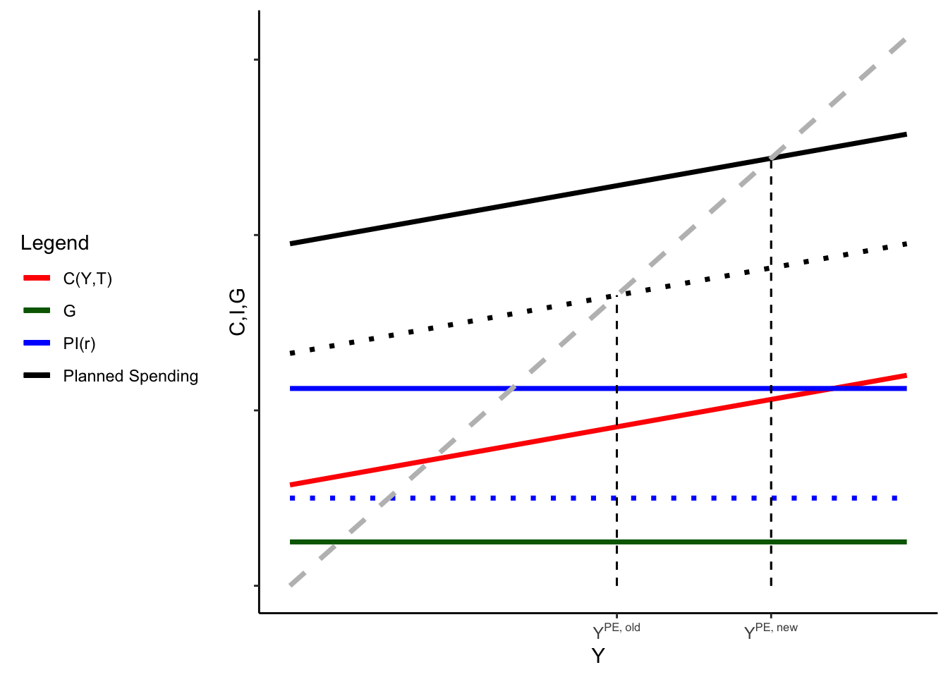
Notice that the increase in \(Y\) is more than we might have expected – in particular, it’s bigger than the increase in \(I\). This isn’t just because of a trick of how the graph is generated, but actually a result of the model.

Exercise:. Using the consumption function and the (mathematical) definition of partial equilibrium, show algebraically that \(Y^{PE}\) is equal to

\[Y^{PE} = \frac{1}{1-b} \left(a -b \times T + I + G \right)\]

Exercise:. Show algebraically, that the increase in investment is smaller than the overall increase in \(Y^{PE}\); that is, \(\Delta Y^{PE} > \Delta I\). This result is what we’d call the “partial equilibrium investment multiplier”. (Hint: write the \(Y^{PE}\) expression in terms of changes, as in the appendix)

The mechanism behind the multiplier is the fact that, in this model, an increase in investment causes an increase in \(Y\), but an increase in \(Y\) feeds back into \(C\), which feeds back into \(Y\) again, etc.

This is unlike the Solow model, where we assumed output was essentially fixed, and changes in \(I\) were 100% offset by a change in \(C\). Here, the components of final demand determine \(Y\).

Exercise:. In the previous exercise, you showed that the multiplier effect depended on the parameter \(b\) of the consumption function. Explain the economic intuition for why a larger propensity to consume implies a larger multiplier effect

As you might expect, there are also fiscal policy multipliers in this model – changes in \(T\) and \(G\) have multiplier effects.

Exercise:. Derive an expression for \(Y^{PE}\) in terms of \(b\) and $T, \(\Delta G\) and \(\Delta I\). What are the multipliers for a change in \(T\), all else equal? What about a change in \(G\), all else equal? What is the economic story for each?

Exercise:. We’ve assumed that \(r\) isn’t changing for these partial equilibrium results. Suppose that there is an increase in \(r\). All else equal, what happens to \(Y^{PE}\)? Graph the relationship between \(r\) and \(Y\), with \(r\) on the vertical axis and \(Y\) on the horizontal axis.

This relationship is where we’re starting in the next section!