2 Partial equilibrium and the “Keynesian Cross”
You probably noticed that, in the last section, \(C\) depended on \(Y\). But we also know that \(Y\) depends on \(C\). So you’re probably wondering how to deal with the circular nature of what we’re doing. That’s what this section is about.
We will assume (temporarily) that real interest rates \(r\) are fixed. In the real world, \(r\) changes of course – we’ll get to it in a bit!
We’ll define planned spending as consumption plus planned investment plus government purchases:
\[ \text{Planned Spending}(Y,r, T, G) = C(Y,T) + PI(r) + G \]
We will define partial equilibrium as the situation where planned spending is equal to actual spending, \(Y\). Formally:
Definition 2.1 Definition of Partial Equilibrium Given an interest rate \(r\), a level of lump sum taxes \(T\) and a level of government spending \(G\), the economy is in partial equilibrium when the following is true:
Consumers are behaving according to their consumption function \(C(Y,T)\)
Given the interest rate, planned investment is described by the investment function \(PI(r)\)
There is no unplanned investment, so: \(I(r) = PI(r)\) and hence \[\text{Planned Spending}(Y^{PE},r, T, G) = Y^{PE} = C(Y^{PE},T) + PI(r) + G \]
This is “equilibrium” because we’re considering what all of the agents in the economy do optimally given a fixed interest rate when they have no reason to change their behavior. But we have not specified how interest rates are determined, which is why we call it “partial.”
What if we were “out of equilibrium?” In that case, there is an unplanned increase or decrease in inventories. Firms would adjust their production accordingly, decreasing production if aggregate spending is too high and pushing it downwards (and vice versa). We’ll focus on the situation where peoples’ plans are consistent with what actually happens and peoples’ behavior is described by the equations we set up.
Exercise:.
Show that, in partial equilibrium, investment is equal to household saving \(S(Y^{PE},T)\) plus public saving \(T-G\). (Use the fact that \(Y = C + I + G\) and \(Y = C + S + T\))Next, we’ll show how to find the partial equilibrium level of output graphically and algebraically.
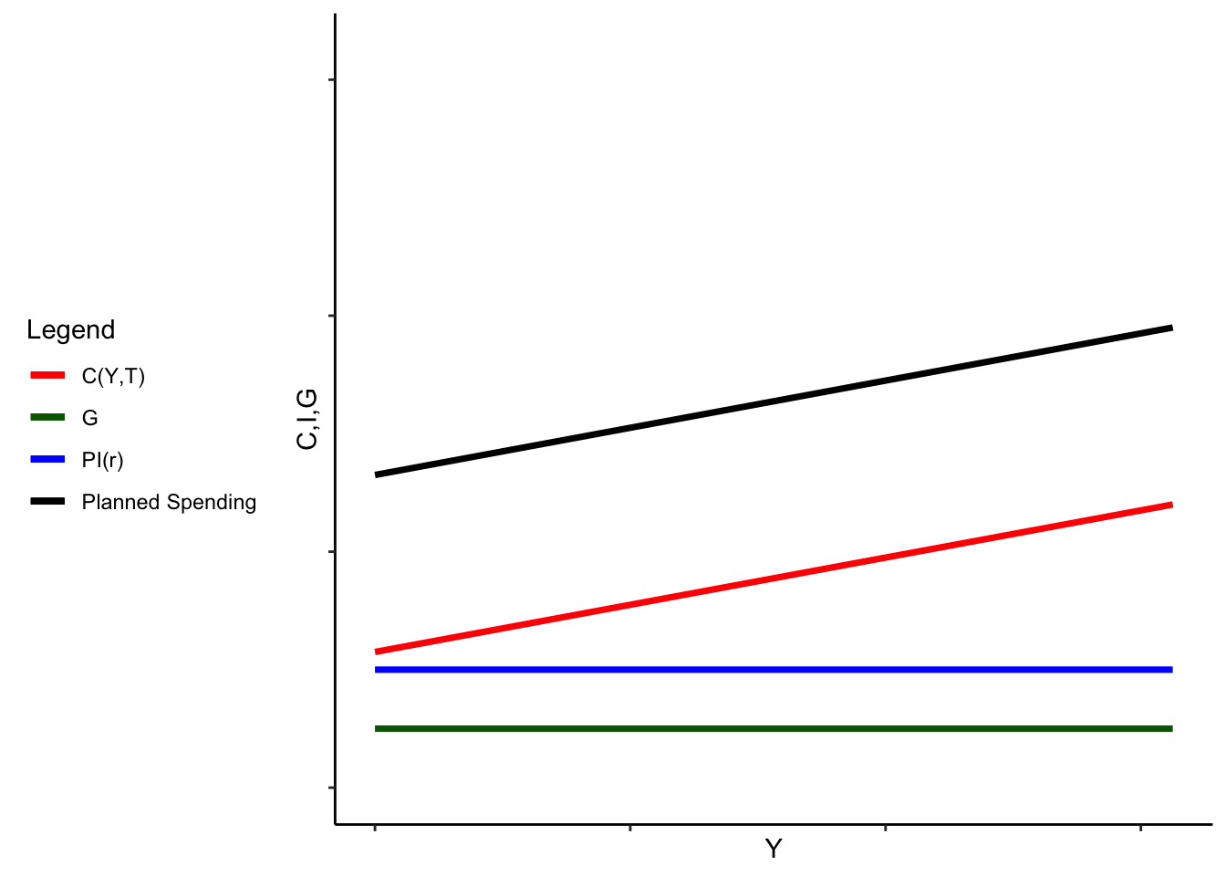
First, graph for planned spending and its components. Notice that because we assumed \(G\) was given, it’s just a number. Similarly, \(r\) is fixed, so \(PI(r)\) is also just a number, and as a result \(G + I(r)\) is just a straight line. \(C\) depends positively on \(Y\) so the consumption function is upward sloping. Since planned spending is \(C + PI + G\), the planned spending function is parallel to the consumption function, but higher.
To find the partial equilibrium level of output, we use a graphical representation called the “Keynesian cross.” Plotting planned spending as a function of \(Y\), and then drawing a 45 degree line out of the origin of the graph. This 45 degree line is like the line \(Y=Y\) - it increases by \(1\) every time \(Y\) increases by \(1\). These graphs will intersect at one point, which is the only point where \(Y = PS(\cdot)\). But that’s exactly our definition of partial equilibrium!
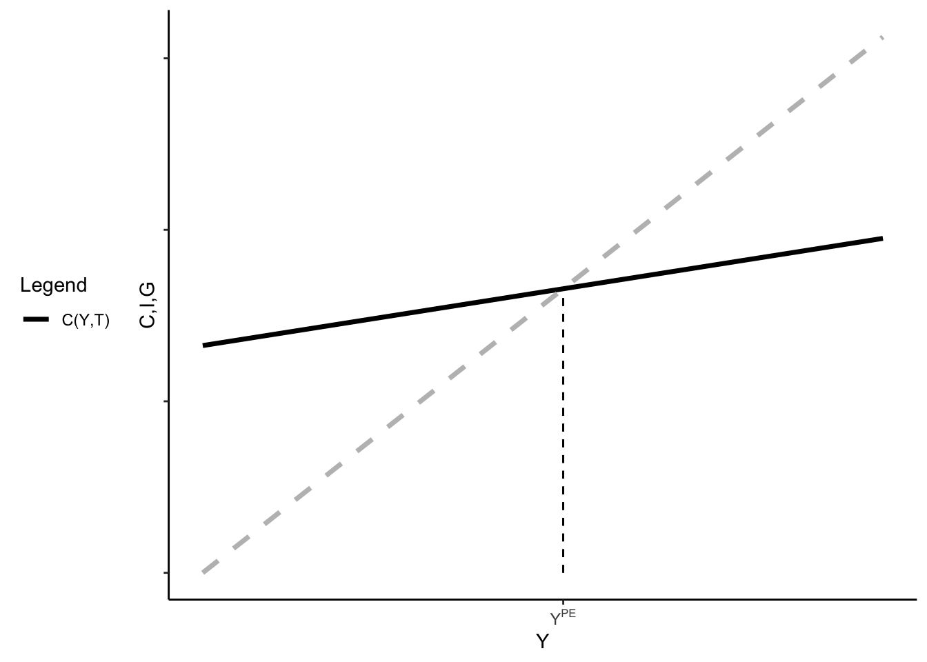
One way of thinking about this is that we know that consumption depends on output and output depends on consumption, etc. There’s one level of consumption and output that are consistent with one another – the intersection of the 45 degree line and the planned spending line.
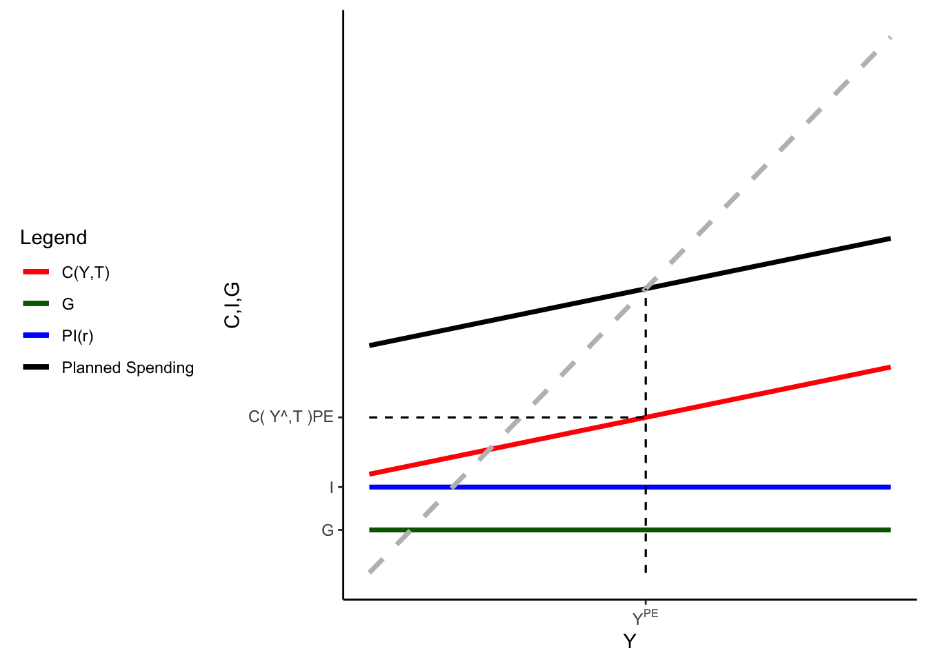
Adding back the components of the planned spending function, we can also show the partial equilibrium levels of the other variables (although for investment and government spending, this is kind of trivial).
Now that we know how to solve the model in partial equilibrium, we’ll show off the multiplier idea.