5 The Monetary Policy (MP) curve

In the previous section, we found a downward-sloping relationship between real interest rates and final demand. In this section, we’ll (finally!) introduce monetary policy to this model.

We showed that monetary policymakers can affect the economy through open market operations. We also discussed that monetary policymakers in the United States typically think about and discuss their policy in terms of a target Federal Funds rate. We will embed this idea into our model.

In theory, the Fed manages the economy by looking through a complicated set of data series and forecasts. However, the economist John Taylor noted that, at least since the mid-1980s, the Federal Reserve’s policy is often summarized through a simple linear relationship. This relationship is now known as the ``Taylor Rule.’’ We’ll assume that the Fed follows a “Taylor Rule” in our model:

Definition 5.1 Assumptions about monetary policy We assume the Federal Reserve sets a nominal interest rate target based on the policy rule \[ i^{FED} = r^* + \pi^* + \alpha \times (Y - Y^{N}) + \beta \times (\pi - \pi^*) \]

\(\alpha > 0, \beta > 1\). \(Y\) is the level of output (GDP), \(Y^N\) is the long run level of output (“potential GDP”), \(Y-Y^N\) is the “output gap”,\(\pi\) is the rate of inflation, \(\pi^*\) is the inflation target, and r^* is the long-run ``natural rate’’ (the real interest rate at \(Y = Y^N\)).

What are some realistic numbers for \(\alpha\) and \(\beta\)? And how well does the Taylor rule describe policy in practice? We can see in the plot below the actual FFR, and the prescriptions of two Taylor rules: One which includes “smoothing” (e.g., the idea that the Fed usually makes small changes to the FFR at any given time) and one that doesn’t (which was Taylor’s original rule).

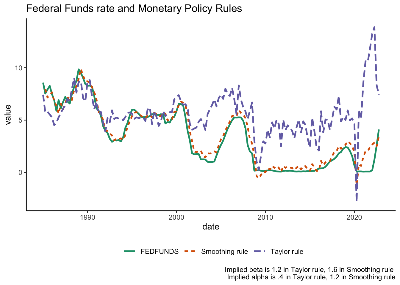
As we can see, the original Taylor rule’s ability to mach the data isn’t perfect. (Some economists, including Taylor, argue that this is a bad thing – they should be following the rule, but aren’t). But a rule of this type does a decent job of matching data in the real world (if we add some smoothing). Since our model doesn’t have any dynamics in it – it’s purely static – it’s okay to focus on the output gap and inflation gap terms.

However, we will modify the rule in two respects. First, notice that the Taylor rule tells us about nominal interest rates, but the IS curve is in terms of real interest rates. We can adjust nominal to real by subtracting inflation. Second, we will add a “shock” term to the rule. The resuling equation is the monetary policy curve, or MP curve.

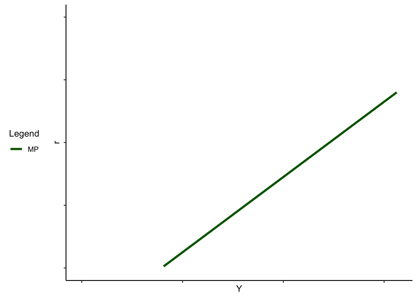
Definition 5.2 Definition of MP curve

The interest rate \(r\) set by monetary policy is \[ r = r^* + \alpha \times (Y - Y^{N}) + (\beta - 1) \times (\pi - \pi^*) + \epsilon \]

\(\epsilon\) is a “shock” term. It captures all the reasons real interest rates might be different from what the Taylor rule prescribes, including monetary policymakers violating their own rule, or financial market conditions which lead interest rates to change at a given level of output.

Now, you might be able to see why we wanted to assume that \(\beta > 1\) in this expression. If \(\pi\) increases by 1%, then \(\beta > 1\) implies that the fed will increase nominal interest rates by more than 1%. This means, by the Fisher equation, \(r\) increases. The response of the Fed to an increase in inflation is to raise real rates, an idea known as the “Taylor Principle”.

Exercise:. Graphically, what is the effect of an increase in \(\epsilon\)? An increase in \(Y^N\)? An increase in \(\pi\)?