6 The Aggregate Demand (AD) curve
The IS and MP curves are a relationship between real interest rates and output. But they also link output and inflation which is the other key business cycle variable we’re interested in – how does the overall change in prices affect real quantities, if at all? The classical model suggested it didn’t, and we’re finally in a position to examine that question with this demand-driven model. The MP curve relates interest rates to inflation, and the IS and MP curves relate output to interest rates.
6.1 Graphical equilibrium
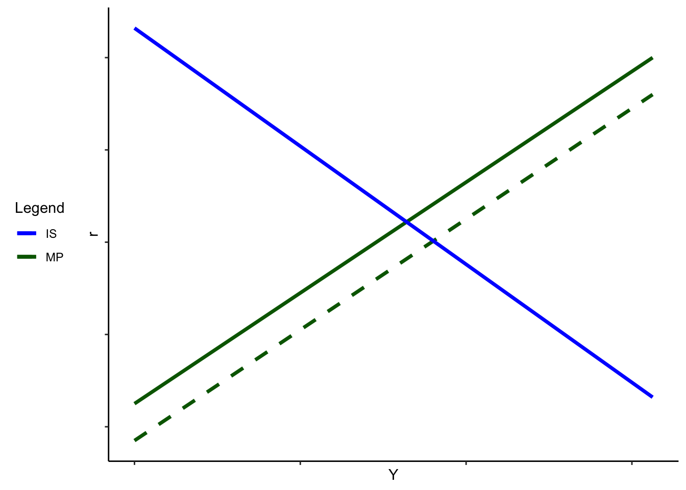
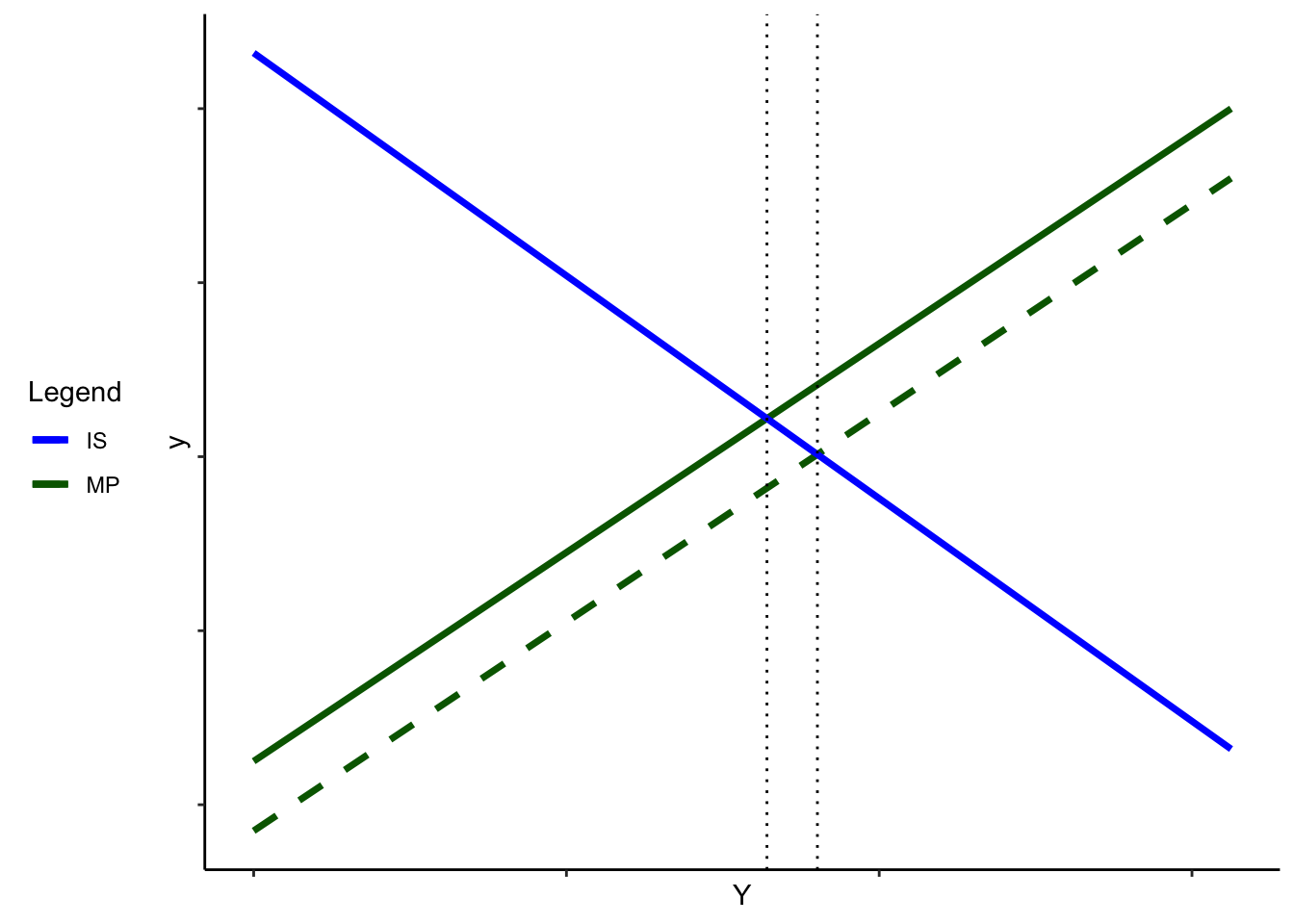
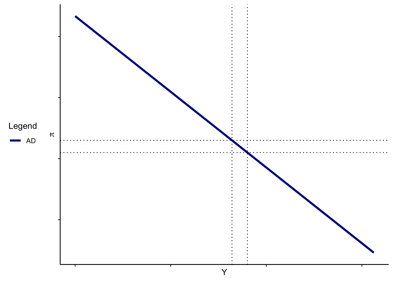
In particular, the equilibrium between IS and MP shows \(Y\) and \(r\) for a given \(\pi\). When \(\pi\) changes, that will shift the MP curve, and hence change \(Y\). That means, holding fixed all the other stuff that shifts IS and MP, we can trace out a relationship between \(Y\) and \(\pi\)

When inflation increases, the MP curve shifts up – at a given \(Y\), \(r\) is higher. This increase in \(r\) leads to a decrease in investment (and hence \(Y\), and hence \(C\), and hence \(Y\)….). In equilibrium, \(r\) is higher and \(Y\) is lower, all else equal.
This means that, all else equal, a higher \(\pi\) is associated with a lower level of demand for final goods and services. We call this relationship the aggregate demand (AD) curve.


Exercise:. How would the following affect the AD curve? – An increase in \(G\)
– An increase in \(T\)
– An increase in \(\epsilon\)
– A decrease in desired consumption at any level of income (a fall in \(a\))
Because the road to this point has been a little winding, it’s worth reminding ourselves of the overall plot.
- The consumption and investment functions, along with given fiscal policy variables, give tell us what level of spending on goods and services is consistent with agents’ investment and savings decisions at any given \(r\).
- The monetary policy rule tells us what level of \(r\) is consistent with the Fed’s policy actions, given \(Y^N, \epsilon\) and, critically, \(\pi\).
- Equilibrium between the IS and MP curves tells us what level of \(Y\) and \(r\) we have for a given \(\pi\). This is a single point on the aggregate demand curve; it tells us what the final demand for goods and services is, consistent with economic agents’ actions.
- But if inflation changes, the Fed changes interest rates. In particular, the Fed raises interest rates when \(\pi\) goes up. This, all else equal, lowers the equilibrium level of \(Y\).
- The end result is that the aggregate demand curve is downward sloping – higher \(\pi\) is associated with lower \(Y\).
In other words, the AD curve slopes downward because of our assumptions about how the Fed reacts, and because of our assumptions about how IS is determined.
We could change the story; problem set questions will ask you to change a number of the assumptions and see how that does (or does not) affect the aggregate demand curve.
6.2 Analytical results
Because our model is relatively simple – it’s linear after all! – we can solve for the mathematical expression for the AD curve.
Exercise:. The AD curve describes an equilibrium relationship between the IS and MP curves. Using the IS equation:
\[Y = \frac{1}{1-b} \left(a -b \times T + (d - h r) + G \right)\] and the MP equation \[ r = r^* + \alpha(Y - Y^N) + (\beta - 1)(\pi - \pi^*) + \epsilon \]
Show that the AD equation is
\[ Y = \frac{1}{1-b+h\alpha} \times \left[ a - bT + d + G - hr^* + h \alpha Y^N - h(\beta - 1)(\pi - \pi^*) - h \epsilon \right]\]
Notice that we can also write this in “changes” form. In particular, let’s study the effect of a change in government spending, holding fixed \(T\) and \(\epsilon\), but allowing \(\pi\) to vary.
\[ \Delta Y = \frac{1}{1-b+ h \alpha} \times ( \Delta G - h (\beta -1)\Delta \pi ) \]
Notice that whether a change in \(G\) increases or decreases GDP depends, critically, on the sign and size of \(\Delta \pi\). \(h (\beta - 1)\) is a positive number, and \(1 - b + h \alpha\) is also positive. But the AD curve alone doesn’t tell us how inflation changes – only that an increase in inflation, all else equal, is associated with lower output.
We need an aggregate supply curve to complement our aggregate demand curve. Adding that will allow us to (1) embed a purely real, long-run model as a special case (2) Consider short-term monetary non-neutrality.