8 Equilibrium and graphical analysis
Now that we have aggregate supply and aggregate demand, we can define equilibrium. But we need to be a little careful, because we seem to have two supply curves and one demand curve.
Definition 8.1 Definition of Equilibrium in the AS-AD model
Equilibrium is the level of output \(Y\) and inflation \(\pi\) at the point where the aggregate demand curve equals short run aggregate supply, \(AD = SRAS\).
In the long run, since \(Y = Y^N\), SRAS and AD must intersect at the long-run aggregate demand curve. This is where \(\pi = \pi^e\).
The transition from a short-run equilibrium to the long-run equilibrium occurs either through a change in fiscal or monetary policy (shifting AD) or, if not through policy, through a change in inflation expectations \(\pi^e\).
When we’re analyzing events in the AS-AD model, we should try to be systematic about it, using something like the following procedure: 1. Decide whether the event affects aggregate demand, short run aggregate supply and/or long-run aggregate supply; 2. Shift the appropriate curve, and find the equilibrium level of inflation and output in the short run where AD = SRAS 3. Explain how (1) if policymakers do nothing, inflation expectations adjust; (2) if policymakers act, what they do to shift aggregate demand.
It’s easiest to see how this works through an example.
8.1 Example: A change in aggregate demand
Suppose that investors decided that now was a good time to expand their firms – say, by investing in new factories or equipment. What effect would this wave of optimism have on the economy? Let’s apply the procedure above:
- Firms’ investment decisions affects their demand for investment; hence, this should shift AD. (In the long run, it could arguably affect \(Y^N\), but we can set that aside – remember that capital might take awhile to get running, and it’s okay for this qualitative model to focus on the main, most important, effect). In particular, it likely increases output at any given level of inflation. (I would think of this as a change in the \(d\) parameter of the investment function).
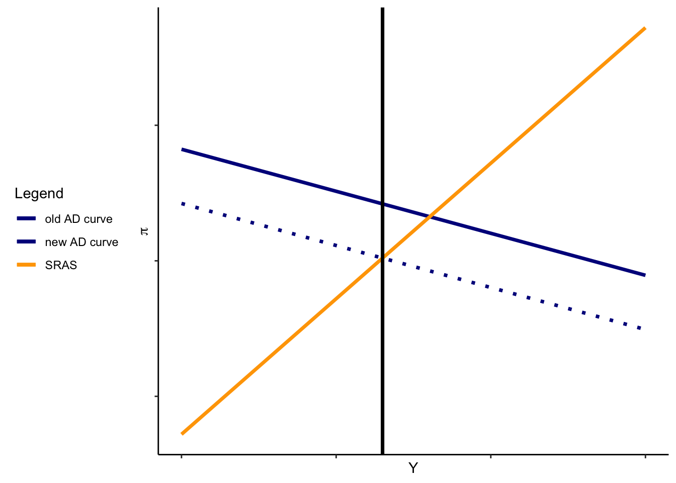
As is clear from the above, the short-run equilibrium is the intersection of the solid blue and orange lines. The expansion in investment raises output, but also leads to an increase in inflation. (The increase in inflation is what induces production to meet the higher demand).
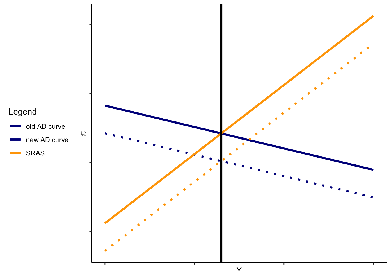
Now, the question is: how do we get back to the long run? If policymakers do nothing (holding \(G\),\(T\),\(\epsilon\) fixed), then the higher-than-expected inflation doesn’t stay higher-than-expected forever. Eventually, workers renegotiate wages to reflect the new high rate of price changes. This reduces the firms’ incentives to produce above potential GDP, shifting SRAS to the left. In the long run, equilibrium is at potential GDP, but with permanently higher inflation.
On the other hand, policymakers may want to avoid higher inflation. If so, they could directly affect aggregate demand by cutting government spending, increasing taxes, and/or engaging in contractionary monetary policy. Any of these could shift AD back to its original position!
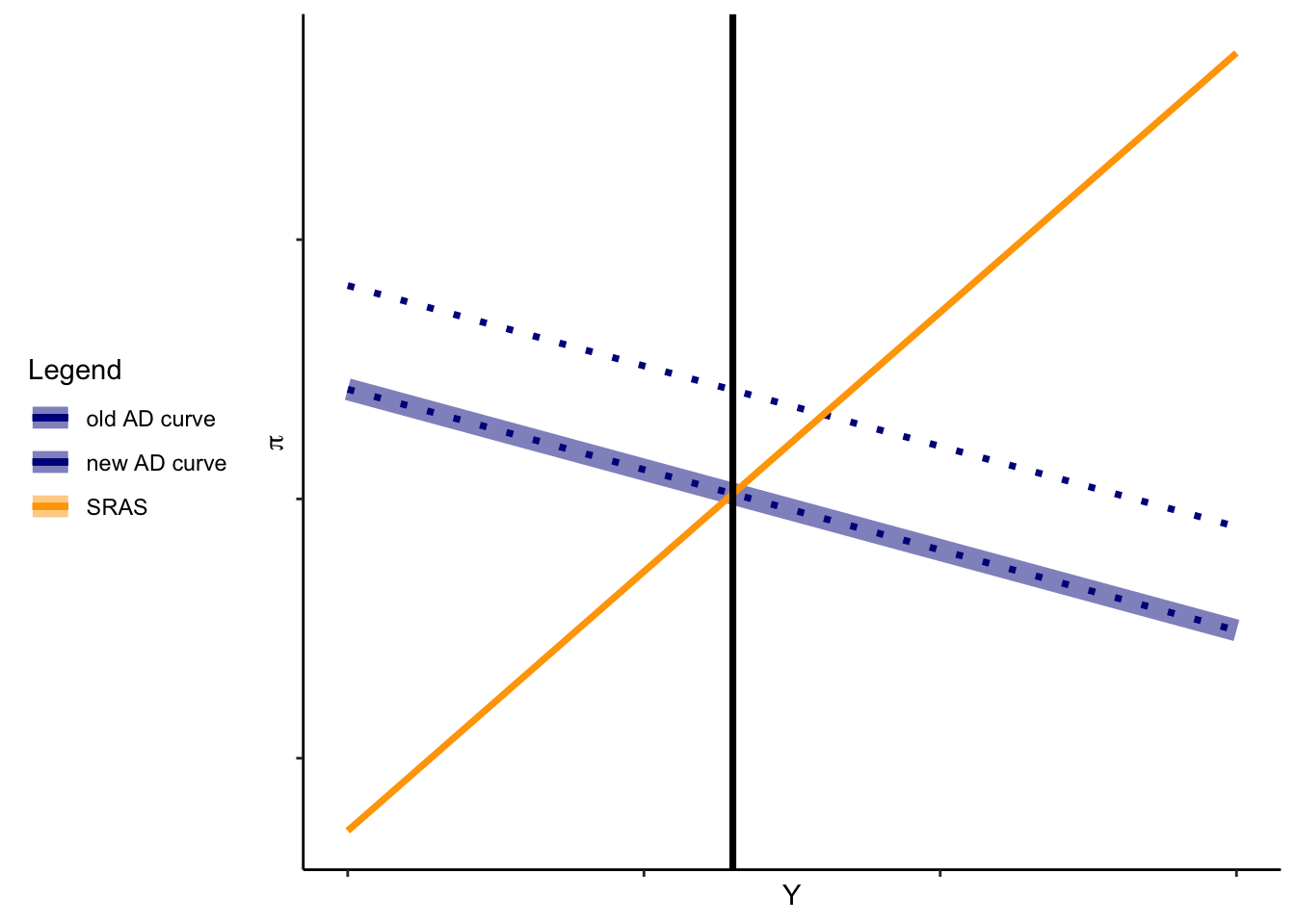
The larger, highlighted line shows the restoration of the original AD curve.