7 Aggregate Supply (AS) and equilibrium

In the last section, we found an expression for aggregate demand:

\[ Y = \frac{1}{1-b+h\alpha} \times \left[ a - bT + d + G - hr^* + h \alpha Y^N - h(\beta - 1)(\pi - \pi^*) - h \epsilon \right]\]

Given $Y$, we could solve for $\pi$. Alternatively, given $\pi$, we could solve for $Y$. But to know what $Y$ and $\pi$ are simultaneously, we need to do a little more work. We’ll develop two versions: one that we’ll call the “long-run” version, which is really a re-statement of the classical model. The second is a “short-run” version, which is closer to what’s in the textbook. Having both versions is helpful because it helps us think about how the short run becomes the long run.

7.1 Long run: the return of the classical model

We already defined $Y^N$ as potential GDP. We can think about this as the level of GDP we expect the economy to return to in the long run, given the quantity of factors of production and production technology.

One way of thinking about the macroeconomy is similar to the classical model: assume that output is determined by $Y^N$, and aggregate demand determines the rate of inflation. This yields a vertical “long run aggregate supply curve.” The macroeconomic equilibrium is determined by the inflation level that, all else equal, keeps output on this long-run aggregate supply curve (graphically, the intersection of AD and LRAS).

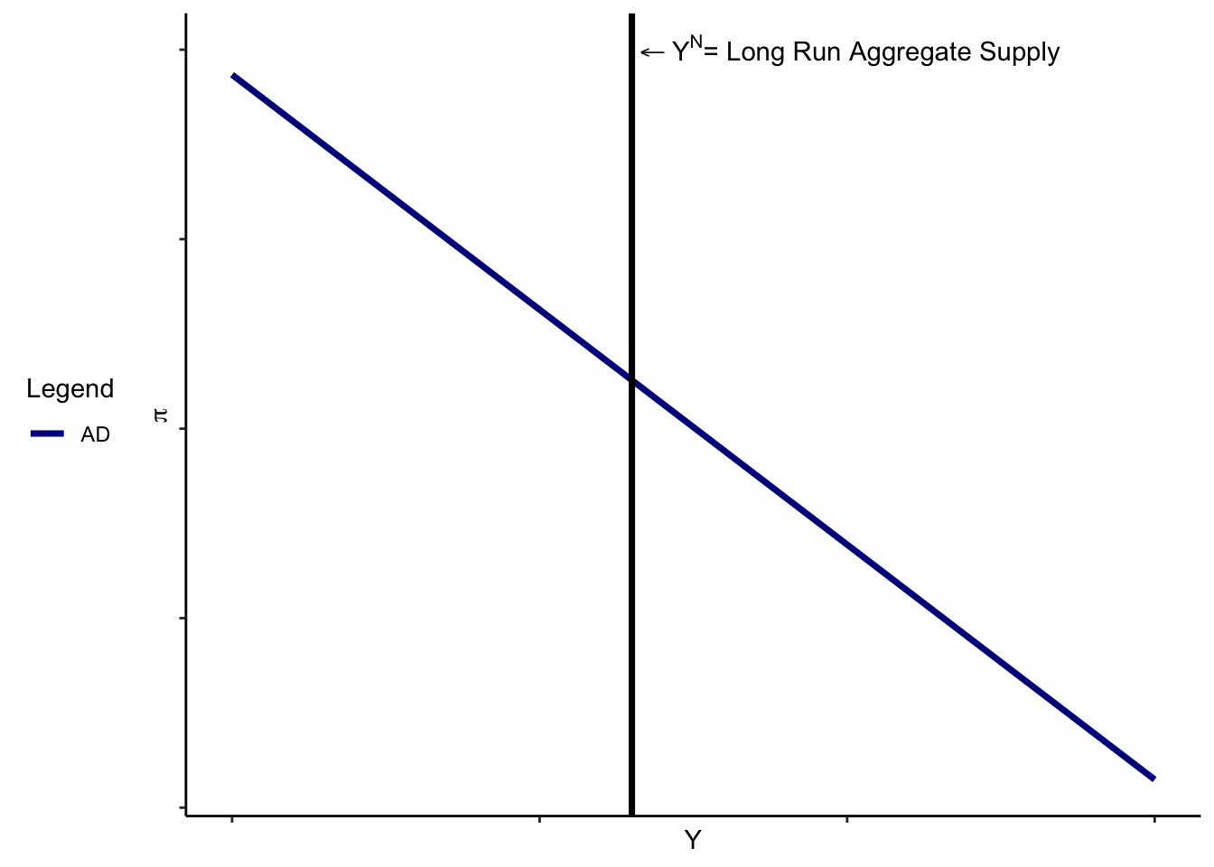
Essentially, the long run aggregate supply curve assumes a particular kind of monetary neutrality: the rate of inflation has nothing to do with the level of output. Aggregate GDP, at the end of the day, must be at the level determined by the available factors of production and technology; prices will adjust to make that the case, and changes to the money supply don’t affect it. A change in aggregate demand may have an effect on what quantities of $C,I,$ or $G$ we end up with, but those also lead to price adjustments so that $Y=Y^N$.

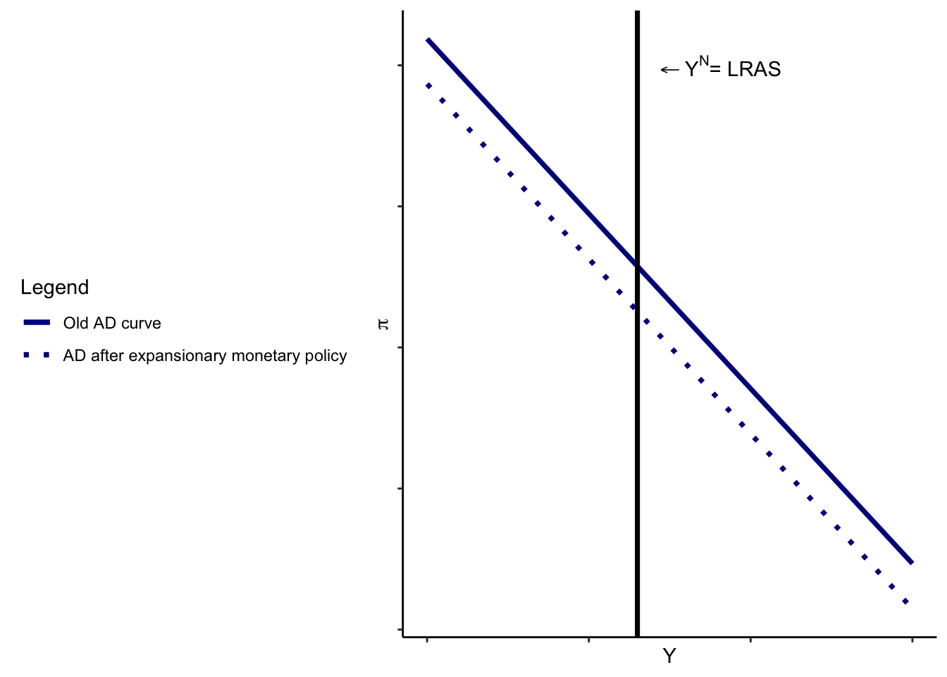
For instance, suppose that the Federal Reserve attempted to increase the money supply. We know from our earlier work that this will, all else equal, lower nominal interest rates. (In terms of model variables, this shifts the MP curve downward without a change in $Y$ or $\pi$ – it’s a decrease in $\epsilon$). But if we are on the LRAS curve, we also know that the increase in money will also be offset by an increase in inflation, which keeps nominal interest rates exactly the same. Real activity is unaffected, prices are higher.

What if a different variable changed? Suppose that $G$ decreased. This would shift AD to the left (at any given level of inflation, output is lower), but the model suggests that inflation would have to fall so that output remains at potential. (Draw it for yourself!)

By emphasizing this as a long-run outcome, we’re essentially saying that aggregate demand determines the rate of inflation, but the supply side of the economy determines output. Government policy that attempts to affect aggregate demand can’t affect $Y$. The government could only affect output in the long run by affecting $Y^N$ – say, by investing in productive capital or choosing policies that result in greater efficiency. These things shift the $Y^N$ curve.

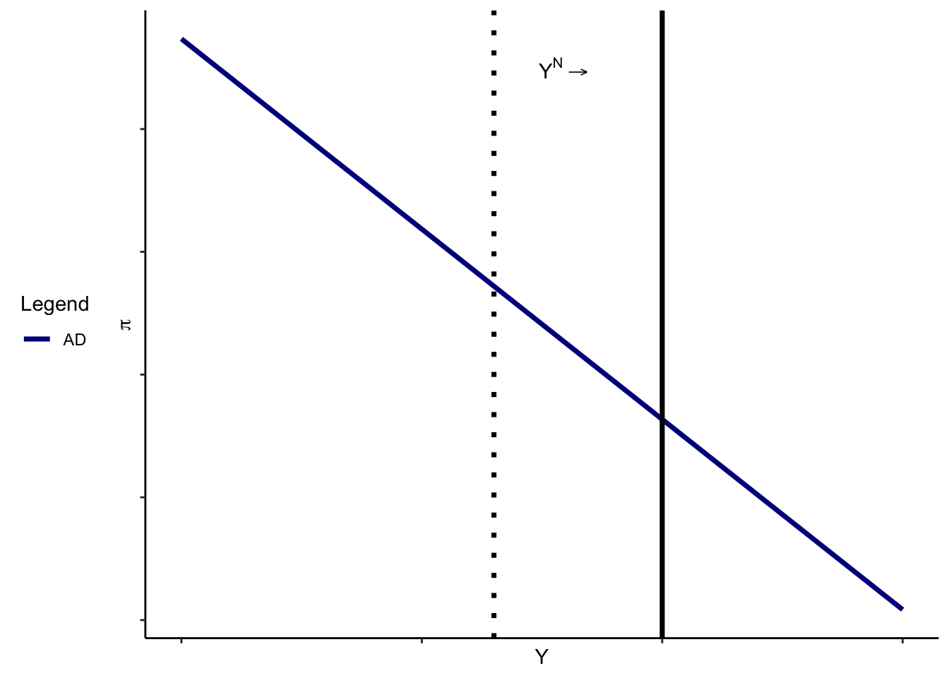
Notice that, consistent with the quantity equation logic, an increase in LRAS (shift to the right, the solid line) will lower inflation if money doesn’t adjust enough to keep that from happening.

The punchline is that the IS-MP-AS (AS/AD) model we’ve developed contains the classical model as, more or less, a special case. However, we need not assume monetary neutrality, and in the next subsection, we’ll relax that assumption. This will allow the economy to be (temporarily) off the long-run aggregate supply curve.

7.2 The Short run

We’ve seen reasons to expect monetary neutrality doesn’t hold at all times. Here, we’ll relax the assumption of pure neutrality by focusing on one possible story: that wages do not adjust freely. (This was one story that Keynes proposed, and while it is not the only possible one, it’s fairly intuitive).

To generate intuition: Suppose we have profit-maximizing firms who hire workers as one possible input into production. Over short horizons, it’s not possible to adjust all of their factors of production, but if they want to adjust how much they produce, they can hire or fire workers. The fact that some factor of production – say, the number of computers and desks available for workers – is fixed means that they face diminishing marginal returns to labor.

The firm decides whether to hire or fire a worker (or, to have a worker work an additional hour) by comparing the benefit to the firm – the marginal revenue generated by the worker for an hour of work – to the marginal cost – the wage. If the worker produces $200 in revenue in an hour of work, and they cost $15 an hour, it is “worth it’’ to the firm to hire them – they keep $185 in profits.

Diminishing marginal returns implies that the amount produced by each worker falls as the number of hours of work increases, so at some point, we have the condition \[ \text{Price of the firm's output} \times \text{Marginal Product of Labor} = \text{Wage} \]

Now we introduce the idea of sticky wages. Suppose that wages are negotiated on infrequently – the worker and the firm agree to a contract that says the worker will receive $15 in nominal dollars for every hour of work, and the contract is re-negotiated every year. That means that the right-hand side is fixed in advance. How do firms and workers negotiate? Well, part of what will affect their negotiations is the real wage they expect – that is, how much they expect inflation to change between now and their next contract. Call $\bar{\text{W}}(\pi^e)$ the fixed nominal wage they negotiate on as a function of $\pi^e$, the expected rate of inflation. Profit maximization implies:

\[ \text{Price of the firm's output} \times \text{Marginal Product of Labor} = \bar{\text{W}}(\pi^e) \] Now, what happens if prices in the economy generally change? The price of the firm’s output is one of those prices – so if $\pi$ is rising, then we’d expect the price of the firm’s output to go up. That implies firms are getting a good deal – they’re earning more revenues, but the cost of workers isn’t changing. (Real wages are going down!). What should they do in that case? Hire more workers! But hiring more workers means the marginal product of labor will fall over until the benefit of hiring workers is equal to the cost.

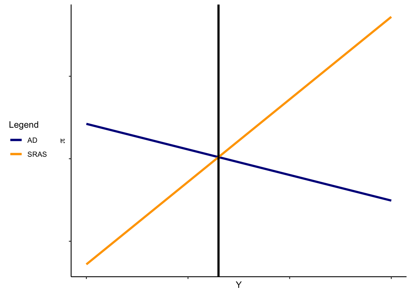
This holds for a single firm. Over the entire economy, we’d expect that the timing of wage negotiation, its flexibility, etc, might differ for different firms. So, handwaving a little bit, we’ll summarize the relationship between prices and production as follows: When inflation is higher than expected, firms have a greater incentive to produce. We summarize this relationship in the following expression:

\[\text{SRAS:} Y = Y^N + \kappa (\pi - \pi^e) \]

$\kappa$ (a greek letter ‘kappa’) is greater than zero, and summarizes how much firms produce above potential when prices are unexpectedly high (and vice versa). If $\kappa$ is large, output is very responsive. On the other hand, the limiting case is when wages also respond perfectly to price changes, in which case $ Y = Y^N$ always and $\kappa = 0$.

Over time, inflation expectations adjust, workers re-negotiate wages, and firms will once again produce at the “natural’’ sustainable level.

To sum up:

If wages are sticky, and are set by firms’ price expectations
then when inflation is higher than expected, firms marginal costs are not increasing, but their marginal benefits are
so they want to produce more.
The adjustment of inflation expectations, and the related setting of wages, brings the economy back to the long-run level of production where $Y = Y^N$.

What shifts short-run aggregate supply? We’ve got two possibilities: (1) Changes in the long-run level of production in the economy of firms (that is, changes in $Y^N$) and (2) changes in firms’ expectations about inflation, holding fixed the actual level of inflation ($\pi^e$).

Let’s dig into that second one. If firms and workers expect that prices will increase in the future, then wages go up today (when they negotiate). However, firms’ prices haven’t actually increased yet. So firms are paying a higher cost without getting a higher benefit; optimally, they cut back on production. All else equal, an increase in expected inflation shifts SRAS to the left.