3 The Investment-Savings (IS) curve

In the previous section, we saw that changes in fiscal policy and investment can have a pretty powerful effect on output (and consumption). But we made the unrealistic assumption that interest rates were fixed. We also showed that an increase in \(r\) would, all else equal, be expected to decrease \(Y^{PE}\).

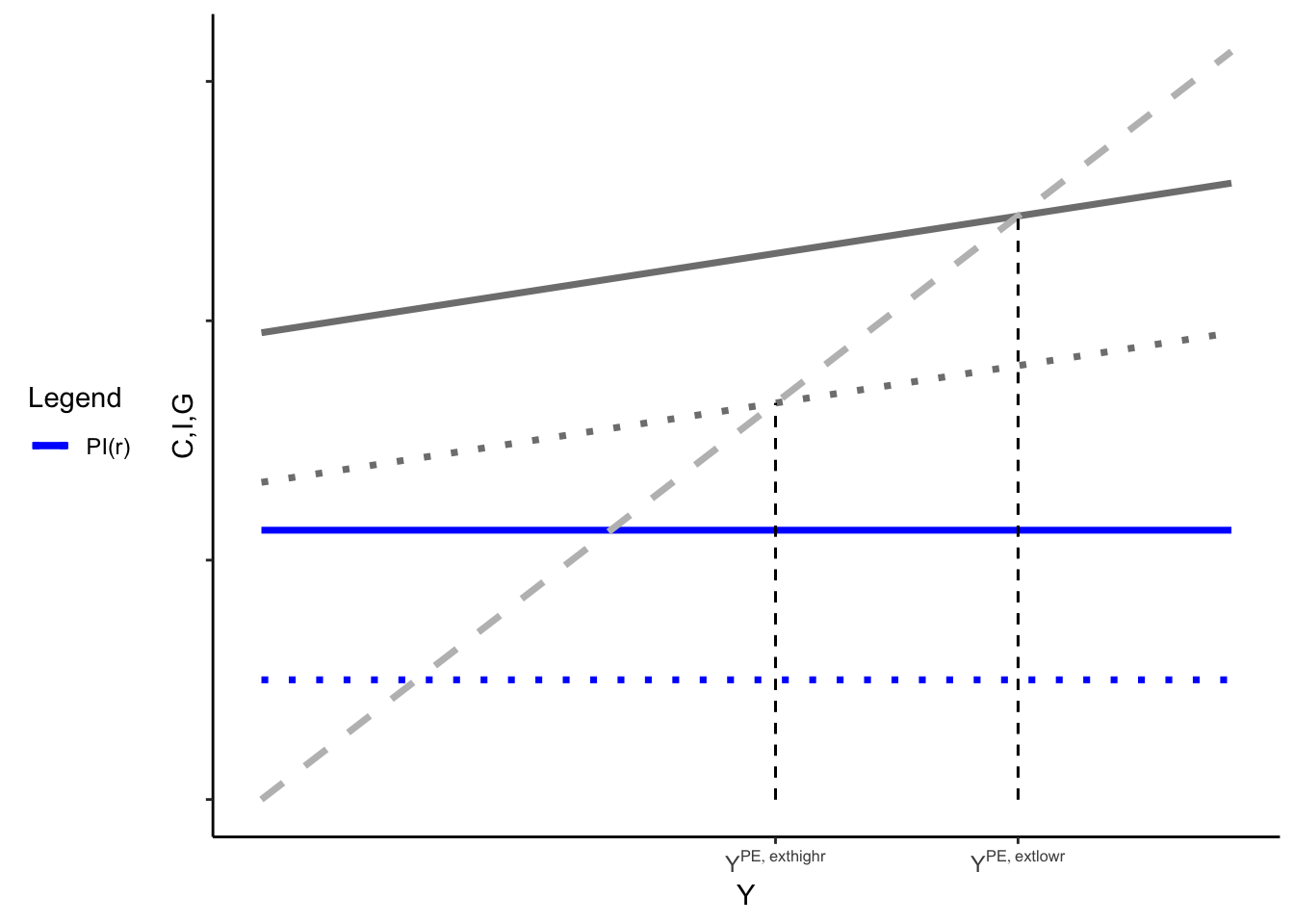
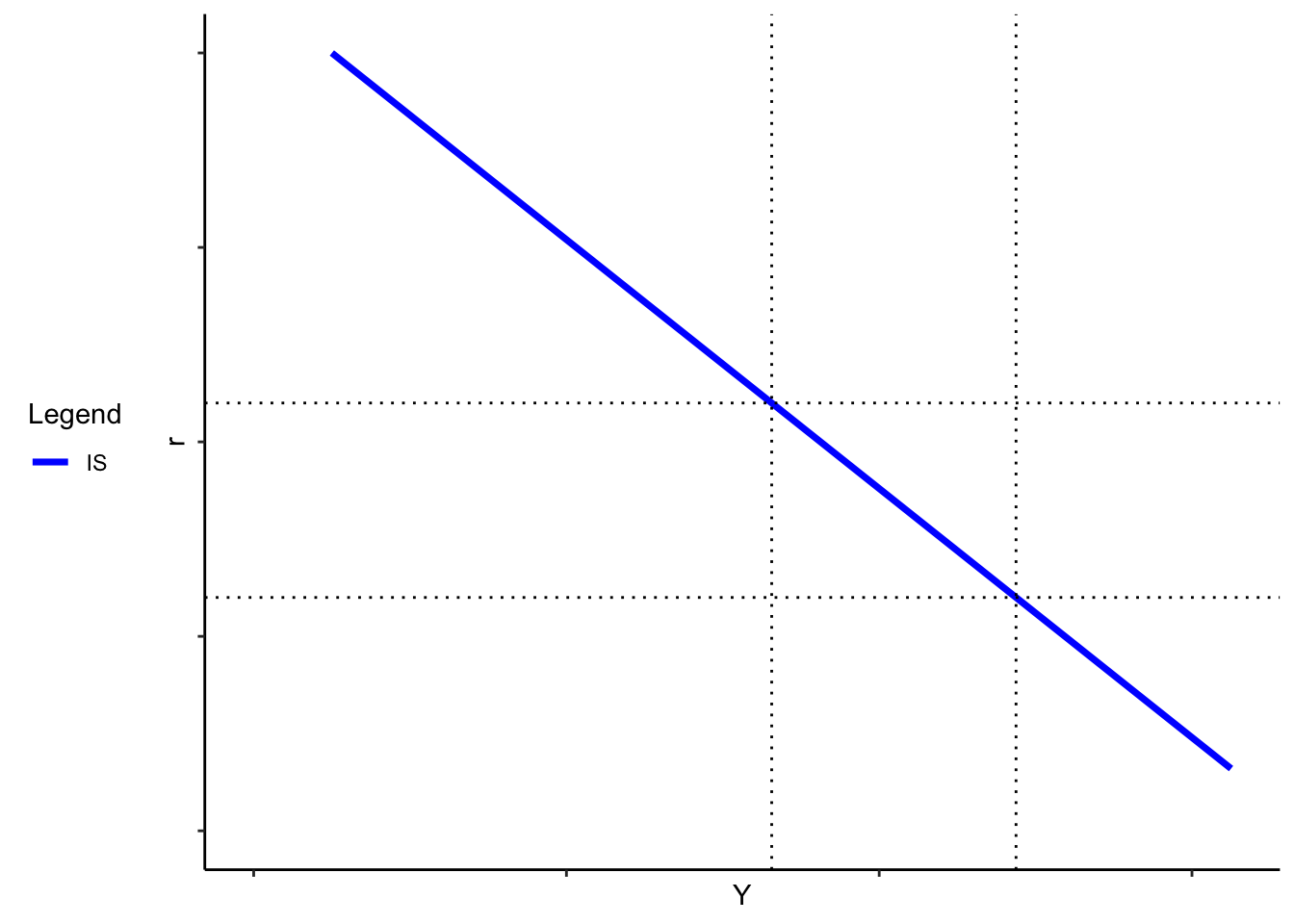
The negative relationship between the \(r\) and \(Y\) is the “Investment-Savings curve” (IS curve). It tells us what the equilibrium level of output is for a given \(r\). (It’s called this because it reflects a particular equilibrium between investment and aggregate savings. A given \(r\) changes investment; we need savings and investment markets to clear, and only one \(Y\) will do it, all else equal).

As you might expect, changes in \(r\), all else equal, lead to movements along the IS curve. Changes in other variables, holding \(r\) fixed, shift the IS curve.

Exercise:. Using the graphical steps you used to to derive the IS curve for a given level of government spending, show graphically what happens when \(G\) falls.

We could also assume that \(I\) is a linear function of real interest rates, that is

\[I = d - h r\]

In this expression, \(h\) represents how responsive \(I\) is to a change in the real interest rate (so if \(r\) goes down by 1%, \(I\) increases by \(h\) dollars). \(d\) captures other factors that affect investment at any given interest rate – such as confidence or beliefs about the future.

Given that assumption, we can derive an analytical expression for the IS curve.

Exercise:. Show that if \(C = a + b(Y-T)\), \(I = d - hr\), \(Y = C + I + G\) and taking \(G\) and \(T\) as given, then \[Y = \frac{1}{1-b} \left( a + - bT + G - hr \right)\]

What is the slope of the IS curve?

The applet below allows you to show (with some numbers attached) how difference choices for each of the parameters affects the IS curve. It’s also available at the following link:IS comparisons app

Notice, however, this is not enough to tell us what \(r\) and \(Y\) actually occur; we have only one curve. Short of assuming the interest rate is always fixed, we don’t have enough information. In the next section, we’ll introduce another curve to pin down \(r\) and \(Y\).