4 Comparing two countries

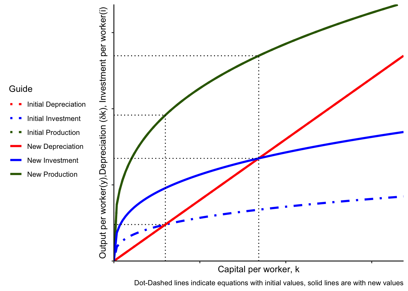
So a few things to remember when doing this kind of exercise: 1. All the curves should always come out of the origin – without capital, we don’t produce. 2. Changes in capital per worker will be movements along the curve, and changes in other variables rotate the curves upward or downward. n this case, a higher savings rate implies that at any given level of \(k\), \(i\) is higher (because \(i = \gamma y = \gamma f(A,k_t, h)\)). \(\gamma\) doesn’t appear in any other equation, so none of the other curves move. Intuitively, the depreciation curve shouldn’t change because it’s only describing how many machines wear out through production; the production function doesn’t change because it just says how much we produce given the inputs available, not what we do with them.

The higher-saving country will have higher capital per worker in the steady state (because they are saving enough to offset a higher level of depreciation), and hence higher output per worker. However, they will not necessarily have higher consumption per worker. Saving more means consuming less at any given level of output. Output is increasing, but so is saving. So, it depends on which change is relatively larger. In the above graph, it is in fact the case that consumption per worker goes down despite output per worker increasing quite a bit.

Increasing saving means the workers in this country face a tradeoff between lower consumption today in favor of higher output tomorrow. Depending on how much they’re saving, they may or may not have higher consumption in the future.

To summarize: According to the Solow model, a country that saves more, all else equal, will be able to sustain a higher level of capital per worker and hence have a higher level of output per worker. They may or may not have a higher level of consumption per worker.

4.1 Numerical and graphical comparisons

We already introduced the Cobb-Douglas production function. If we are willing to assume that the Cobb-Douglas function is a good description of production, we can use it to make numerical predictions about the levels of capital per worker (and hence output, investment, and consumption) in different countries by picking different numerical values for the parameters.

Below, there’s an interactive application which lets you select parameters for two countries, , calculate steady state values, and plots the comparative graphs. This may be helpful for checking your work as you practice using the model. It’s also available at the following link: Solow comparisons app