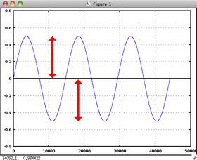
DC = 0 (good)
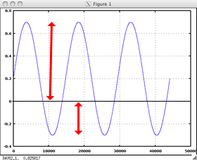
DC = .2 (bad)
An audio effect can be thought of as a black box whose input is an audio signal and whose output is a modified version of that signal. Common digital audio effects are known by the names: amplification, normalization, reverb, distortion, flanging, chorusing, compression, limiting, enhancing, equalize, parametric equalizers, and delay lines. The signal can be processed mathematically (software) or electronically (hardware). Some effects are subtle and some effects are obnoxious. Software effects can be classified as time domain effects or frequency domain effects. Time domain effects manipulate the actual samples. Frequency domain effects take the FFT of the signal, modify the frequency spectrum, and then convert the modified spectrum back into the time domain with the IFFT.
Many of the time domain effects have their origins in the days of analog tape studios. The audio signal was recorded onto magnetic tape and played back through a tape deck. Effects were produced by speed changes, playing the tape backwards, and cutting the tape into small fragments and reassembling the fragments in a different order. Similar effects are found in virtually all sound editing software programs.
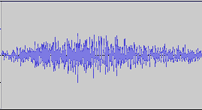
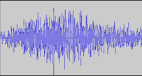
Time domain effects work optimally when the mean of all sample amplitudes is zero. Another way of stating this is that the sum of all positive amplitudes and the the sum of all negative amplitudes should equal zero. The term DC stands for "Direct Current". In electronics and analog synthesizers you could and a small amount of current to a waveform to balance its symmetry above or below the x axis. In digital audio you want the DC line to lie right on the x axis. The Remove DC Offset effect should be the first effect used on an audio file.
DC = 0 (good) |
DC = .2 (bad) |
|
|
The Amplify effect raises or lowers the volume of a sound to a specific decibel level. Conversion formulas between amplitude and decibels are shown below.
| Formula | Example | Comments |
| 0.5 is a ratio where the amplitude of one sound is half as that of another | ||
| If one sounds os -6dB softer than another its amplitdue will be half that of the louder sound, on an amplitude scale from -1 to +1. |
The Normalize effect will raise the volume of a sound to its maximum level just short of clipping. You find a scaling factor that when multiplied by each sample brings the maximum amplitude very close to 1.0 and the minimum amplitude very close to -1.0. A Normalized file would be very close to, but should never exceed zero decibels.
Before |
Amplified to -6dB |
Normalized |
 |
|
 |
You studied envelope functions in Unit 10. An envelope amplifies segments of a sound by varied amounts.
The most common method of changing the speed of a sound is to skip samples or play the same sample more than once. This type of speed change affects the pitch as well as the length of the file. Integer speeds are easy. It gets more complicated when you need to change the pitch to a specific frequency. Here's the Music108 sound played at normal speed, half speed, twice the speed, and three quarter speed.
| Speed | Procedure | Sound | Pitch | File Length |
| Normal Speed | Play every sample | normal | 1x | |
| Twice as Slow | Play every sample twice | one octave lower | 2x | |
| Twice as Fast | Play every other sample | one octave higher | 0.5x | |
| 0.75 as Fast | In Unit 11 labs. |
Delay Lines are frequently used in audio software. The technique originated with tape recorder where the magnetic tape was sometimes run through two tape decks whose play heads were a separated by several inches to several feet. A short delay (distance) "fattened" the sound. A long delay sounded like an echo. Multiple decaying delays could simulate reverberation.
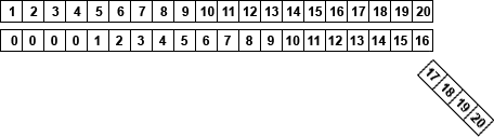
Sound samples are long lists of numbers representing the amplitude of the sound wave at each sample point. These sequential lists of amplitudes are often called arrays, vectors or lists. This picture represents the first twenty samples of the sound.
![]()
By adding zeros at the beginning of the sound, you can delay the start. A ten millisecond delay would add 441 zeros. This picture shows the sound delayed by four samples.
![]()
In Octave, before you can add the delayed samples and the original samples the two vectors have to be of equal length. Either the delayed waveform will need to be truncated, or an equivalent delay will need to be added to the end of the original waveform. This picture illustrates truncation, four zeros were added at the beginning, four samples were chopped off at the end.
Delay times can be measured in samples, but they're usually measured in milliseconds or seconds. Tempo delays are calculated as a fractions of a beat. Delay times can be categorized as:
Three sound files will be used to illustrate the different delay times. The Violin pizzicato sounds have a sharp attack and almost no sustain. The cello sounds have a smooth attack and long sustain. The third sound is speech. The melody played by the violin and cello is one I created for this example.

| Instrument | Original Sound |
| Violin Pizzicato | |
| Speech | |
| Cello |
Short delays range from a few samples to a few milliseconds, generally less than 10 ms and are sometimes used to compensate for phase issues in stereo recordings. If two microphones are more than a few inches apart, sounds reach the left and right microphones at different times and can cause phase cancellation. By calculating the distance between the microphones and knowing the speed of sound, you can calculate the number of samples needed to delay one of the signals in order to reduce the phase cancellation problems.
| Instrument | Delayed Sound - 8 ms |
| Violin Pizzicato | |
| Speech | |
| Cello |
Medium delays in the rage of 10-50 milliseconds have the effect of "fattening" a signal.
| Instrument | Delayed Sound - 45 ms |
| Violin Pizzicato | |
| Speech | |
| Cello |
Medium delays in the range of 60-100 milliseconds are sometimes called Slapback echoes.
| Instrument | Delayed Sound - 80 ms |
| Violin Pizzicato | |
| Speech | |
| Cello |
Delays longer than 100 milliseconds are heard as distinct echoes.
| Instrument | Delayed Sound - 150 ms |
| Violin Pizzicato | |
| Speech | |
| Cello |
This effect is caused by mixing multiple delays at different time intervals.
When delays follow the tempo they're known as Tempo Sync Delays. This example was tempo sync'd to the 16th note.
| Notes | Pattern | Sound |
| 12 | ||
| 13 | ||
| 14 | ||
| 123 | ||
| 124 | ||
| 134 | ||
| 234 | ||
| 1234 |
A form of reverb can be created using multiple delays with each delay decaying exponentially. Here's an example using 6 delays spaced 100 milliseconds apart. The initial gain is around 0.9. Each successive delay 0.9^n.
| Instrument | Comb Filter Reverb |
| Violin Pizzicato | |
| Speech | |
| Cello |
Three common methods of rearrangement are reversal, splicing and looping. Reversing the sound on tape was easy, just play the tape backwards. With digital audio you just play the samples in reverse order. Tape splicing involved recording multiple copies of one tape and then cutting the copies into small pieces, rearranging the pieces and splicing them back together to form a new tape. A tape loop could be created by splicing the ends of the tape together so it would play continuously.
Here are some sound clips played in reverse. Some sounds are affected more than others.
| Normal | Reverse | |
| FM brass | ||
| Piano | ||
| FM drums | ||
| Guitar | ||
| Saxophone melody | ||
| Speech |
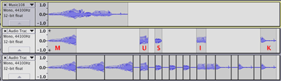
Morphing is a form of splicing where combine the a attack portion of one sound, the sustain portion of another sound, and apply the release portion of a third sound to create a new sound. This example uses the attack of a guitar, the steady state of a piano, and the release of a violin.
Splicing can create a stutter effect by copying small segments of a file and pasting them one or more times to create a different arrangement.
 |
Track 1 Normal | |
| Track 2 Slices | ||
| Track 3 Stutter |
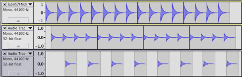
When you repeat a sound over and over it's called a sound loop or simply a loop. In this example a single FMdrum sound was copied (looped) four times exactly 44100 samples (one second) apart. That one measure was copied four times to create a four measure loop. The four measure phrase could be looped to create an eight measure phrase, etc. The second track is a copy of the first delayed by one half beat and reduced in amplitude by -6 dB. The third track is a copy of the second delayed by an additional one quarter beat and further reduced in amplitude by -3 dB. Beats 1 and 3 were deleted in track three.
 |
The point where the waveform crosses the X axis is known as a zero crossing point. You want to join file segments together at zero crossing points. Otherwise the discontinuity will create a click.
Revised John Ellinger, January - September 2013